About pagination
What is pagination? What is it good for? Let’s imagine we have a database that hold data about users and we have a lot of user. If a front end application would like to display it on a website, then it must fetch from database. In a good scenario, front end does not reach the database directly, but instead reach an backend server (e.g.: REST API backend) who has connection with database to fetch data.
Now the question: when we want to list users on front end, we have to fetch all of data from database? Let’s say we have 100k users in the database. If front end fetch all of it, then it could more problems:
- Increase the network bandwidth between backend and frontend that can result in a slower page load
- Increase the memory usage on the backend because database has to fetch all of the data
So put extra workload to the backend, meanwhile it makes the loading on front end slower. Without real benefit, because no user wants to read such a huge data at once.
Solution for this problem is called: pagination. With this technic, instead of serving all data, backend just serves slices of data. And more data can be fetch later. For example, as user scroll down and reach the last slices of the fetched slice, then front end can request for the next slice.
But how the pagination can be implemented?
Naive solution
Well, nobody know everything at the start line. I have made mistakes in the past (and still do), but I try to learn from my mistakes. And this is one of them. First, I make pagination many years ago, I have done something like:
SELECT * FROM users OFFSET 100 LIMIT 10;
What is the problem here (aside that we don’t do SELECT *, it is just an
example).
When I first tried it, database was small.
I did not feel that this query has major problems.
But as the database has been grown queries has become slower and it has a
major problem.
I have made an EXPLAIN statement to check it.
=> EXPLAIN (ANALYZE, TIMING) SELECT * FROM users OFFSET 1000 LIMIT 10;
                                                     QUERY PLAN
--------------------------------------------------------------------------------------------------------------------
 Limit  (cost=31.96..32.28 rows=10 width=141) (actual time=0.461..0.464 rows=10 loops=1)
   ->  Seq Scan on users  (cost=0.00..31964.00 rows=1000000 width=141) (actual time=0.013..0.388 rows=1010 loops=1)
 Planning Time: 0.089 ms
 Execution Time: 0.484 ms
(4 rows)
What do we see? analysis says that the actual execution time is between 0.461 and 0.464ms. It also showed that it does not use indexes for read but doing a sequential scan on the table. Although it still very fast (under 1ms), but the sequential scan and lack of index usage foresees an issue with higher number of offset.
To validate it, I have run the query with 100_000 offset. The execution time has been increased to ~26ms from ~0.5ms. This is a significant increment!
=> EXPLAIN (ANALYZE, TIMING) SELECT * FROM users OFFSET 100000 LIMIT 10;
                                                      QUERY PLAN
-----------------------------------------------------------------------------------------------------------------------
 Limit  (cost=3196.40..3196.72 rows=10 width=141) (actual time=26.779..26.786 rows=10 loops=1)
   ->  Seq Scan on users  (cost=0.00..31964.00 rows=1000000 width=141) (actual time=0.014..19.625 rows=100010 loops=1)
 Planning Time: 0.087 ms
 Execution Time: 26.808 ms
(4 rows)
Better solution
I don’t say this is the best solution, because best solution really depends on the actual case. In my case, the database is reading in case of 90%, so I focusing on the read performance (thus just testing SELECT). Besides who knows, maybe I learn something in the future which makes this solution not best anymore. So I say this is just a better approach (based on numbers).
What has been changed? Instead of offset, I am using a WHERE clause and filter
for the id (which is a primary key so indexed column). Query looks like:
SELECT * FROM users WHERE id > 100 LIMIT 10;
And let’s see the EXPLAIN result for the higher offset but with WHERE clause.
=> EXPLAIN (ANALYZE, TIMING) SELECT * FROM users WHERE id > 100000 LIMIT 10;
                                                   QUERY PLAN
-----------------------------------------------------------------------------------------------------------------
 Limit  (cost=0.00..0.38 rows=10 width=141) (actual time=0.015..0.020 rows=10 loops=1)
   ->  Seq Scan on users  (cost=0.00..34464.00 rows=901068 width=141) (actual time=0.014..0.017 rows=10 loops=1)
         Filter: (id > 100000)
 Planning Time: 0.114 ms
 Execution Time: 0.041 ms
(5 rows)
It can be clearly seen that it still made a sequential scan, but not the whole
table from the first row, but it sees that id is an indexed column, so first
it makes a index search, then just start scanning.
It is significantly faster then the offset approach even for higher number of
offset.
Its execution time is 0.041ms, comparing with the offset approach, where it was
26.808ms, it means more than 600 times faster execution time!
The boring numbers
The engineer in myself says that 1 measurement does not count. Although, logically thinking, the result is very make sense, but I am curious of its scale and I would also analyze it from memory footprint view as well. I have generated a database with random data with 1 million lines.
The plan for data collection
My plan is to make 50 measure point in every 50_000 between 0 and 999999 offset. 50 measure point reduce the noise as I saw with some test measure. Test collector script looks like:
#!/bin/bash

for i in {0..999999..50000}; do
    for j in {0..50}; do
        psql -U test -d dummy -A -t -c "explain (ANALYZE, BUFFERS, TIMING, FORMAT JSON) select * from users where id > $i limit 10;" >/tmp/measure_id_${i}_${j}.json
    done
    echo "Done with $i for id"
done

for i in {0..999999..50000}; do
    for j in {0..50}; do
        psql -U test -d dummy -A -t -c "explain (ANALYZE, BUFFERS, TIMING, FORMAT JSON) select * from users offset $i limit 10;" >/tmp/measure_offset_${i}_${j}.json
    done
    echo "Done with $i for offset"
done
This script generates 4080 files for each query type. Sample output of above command like this:
[
  {
    "Plan": {
      "Node Type": "Limit",
      "Parallel Aware": false,
      "Async Capable": false,
      "Startup Cost": 30365.8,
      "Total Cost": 30366.12,
      "Plan Rows": 10,
      "Plan Width": 141,
      "Actual Startup Time": 120.915,
      "Actual Total Time": 120.917,
      "Actual Rows": 10,
      "Actual Loops": 1,
      "Shared Hit Blocks": 15907,
      "Shared Read Blocks": 4960,
      "Shared Dirtied Blocks": 0,
      "Shared Written Blocks": 0,
      "Local Hit Blocks": 0,
      "Local Read Blocks": 0,
      "Local Dirtied Blocks": 0,
      "Local Written Blocks": 0,
      "Temp Read Blocks": 0,
      "Temp Written Blocks": 0,
      "Plans": [
        {
          "Node Type": "Seq Scan",
          "Parent Relationship": "Outer",
          "Parallel Aware": false,
          "Async Capable": false,
          "Relation Name": "users",
          "Alias": "users",
          "Startup Cost": 0.0,
          "Total Cost": 31964.0,
          "Plan Rows": 1000000,
          "Plan Width": 141,
          "Actual Startup Time": 0.015,
          "Actual Total Time": 85.248,
          "Actual Rows": 950010,
          "Actual Loops": 1,
          "Shared Hit Blocks": 15907,
          "Shared Read Blocks": 4960,
          "Shared Dirtied Blocks": 0,
          "Shared Written Blocks": 0,
          "Local Hit Blocks": 0,
          "Local Read Blocks": 0,
          "Local Dirtied Blocks": 0,
          "Local Written Blocks": 0,
          "Temp Read Blocks": 0,
          "Temp Written Blocks": 0
        }
      ]
    },
    "Planning": {
      "Shared Hit Blocks": 90,
      "Shared Read Blocks": 0,
      "Shared Dirtied Blocks": 0,
      "Shared Written Blocks": 0,
      "Local Hit Blocks": 0,
      "Local Read Blocks": 0,
      "Local Dirtied Blocks": 0,
      "Local Written Blocks": 0,
      "Temp Read Blocks": 0,
      "Temp Written Blocks": 0
    },
    "Planning Time": 0.563,
    "Triggers": [],
    "Execution Time": 120.962
  }
]
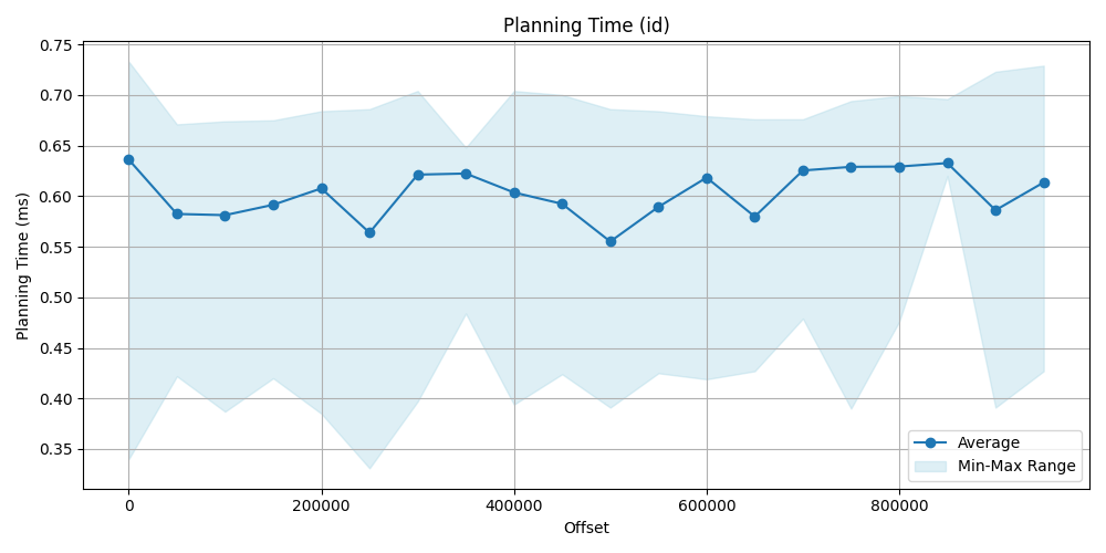
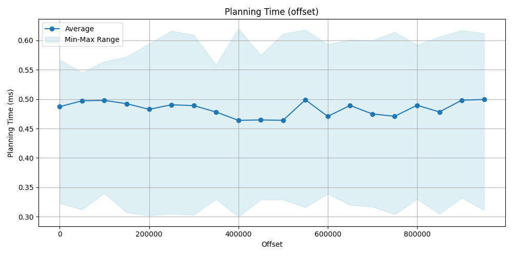
Planning time comparison
The planning time is very similar in both case. For offset approach is a bit faster but insignificant. Conclusion for the planning time that its difference is really insignificant, both are very fast (since these are very simple queries).
| Offset | Avg (id) [ms] | Avg (offset) [ms] | Offset | Avg (id) [ms] | Avg (offset) [ms] | |
|---|---|---|---|---|---|---|
| 0 | 0.636 | 0.487 | 500_000 | 0.555 | 0.464 | |
| 50_000 | 0.582 | 0.497 | 550_000 | 0.589 | 0.498 | |
| 100_000 | 0.581 | 0.497 | 600_000 | 0.618 | 0.470 | |
| 150_000 | 0.591 | 0.492 | 650_000 | 0.579 | 0.489 | |
| 200_000 | 0.607 | 0.482 | 700_000 | 0.625 | 0.474 | |
| 250_000 | 0.563 | 0.490 | 750_000 | 0.628 | 0.470 | |
| 300_000 | 0.621 | 0.488 | 800_000 | 0.629 | 0.489 | |
| 350_000 | 0.622 | 0.478 | 850_000 | 0.632 | 0.478 | |
| 400_000 | 0.603 | 0.463 | 900_000 | 0.586 | 0.498 | |
| 450_000 | 0.592 | 0.464 | 950_000 | 0.613 | 0.499 |
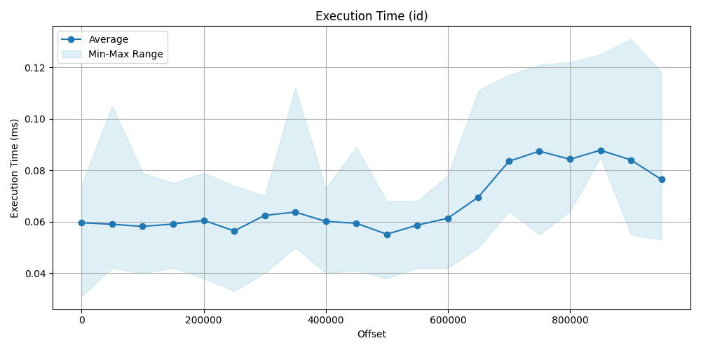
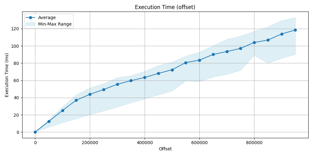
Execution time comparison
This is where the real difference can be seen. On the data point and the plot obviously show, that we have seen earlier and was predictable, that filtering for index then make a sequence scan is significantly faster then a simple sequence scan by using offset, id approach is faster even more hundred times.
| Offset | Avg (id) [ms] | Avg (offset) [ms] | Offset | Avg(id) [ms] | Avg (offset) [ms] | |
|---|---|---|---|---|---|---|
| 0 | 0.0596 | 0.059 | 500_000 | 0.0551 | 72.336 | |
| 50_000 | 0.0590 | 12.486 | 550_000 | 0.0586 | 80.636 | |
| 100_000 | 0.0581 | 25.136 | 600_000 | 0.0613 | 83.507 | |
| 150_000 | 0.0590 | 37.032 | 650_000 | 0.0695 | 90.088 | |
| 200_000 | 0.0605 | 43.822 | 700_000 | 0.0835 | 93.433 | |
| 250_000 | 0.0564 | 49.412 | 750_000 | 0.0874 | 97.098 | |
| 300_000 | 0.0624 | 55.462 | 800_000 | 0.0842 | 103.953 | |
| 350_000 | 0.0637 | 59.697 | 850_000 | 0.0877 | 106.777 | |
| 400_000 | 0.0601 | 63.397 | 900_000 | 0.0839 | 113.861 | |
| 450_000 | 0.0593 | 68.085 | 950_000 | 0.0764 | 118.394 |
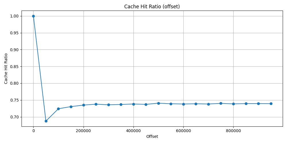
Buffer usage
I have checked two values of the shared block (size of one block is 8k):
Shared Hit Block: It means that the block has been read from memory (RAM) instead of disk.Shared Read Block: It means that the block has been read from the disk.
I was curious that how much extra memory is used by the offset query.
It makes sense that it would use more, but I just wanted to make a number for it.
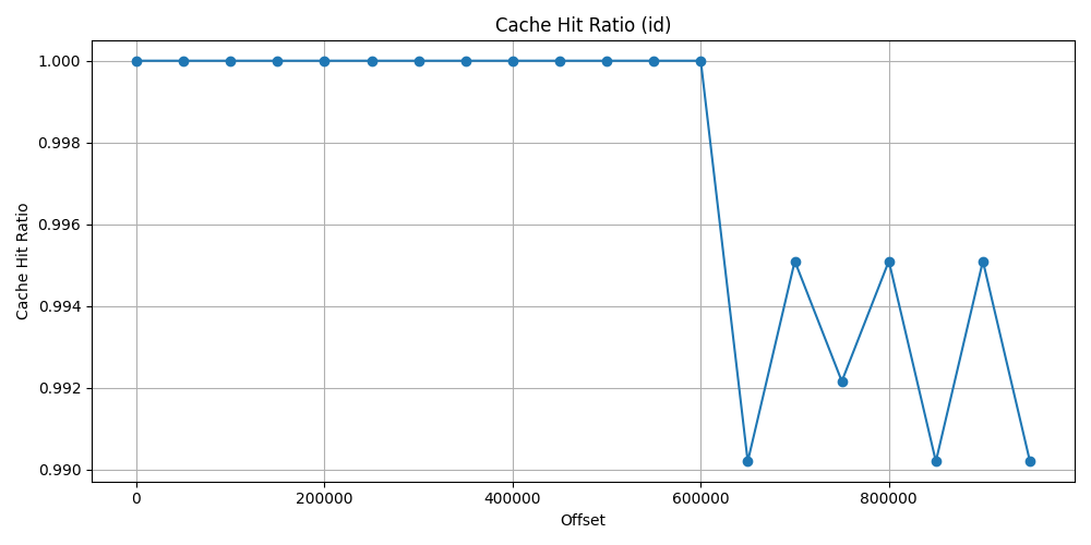
I have made a cache ratio which is: cache_ratio = shared_hit_block / (shared_hit_block + shared_read_block). So in a good scenario it should tend
towards 1.
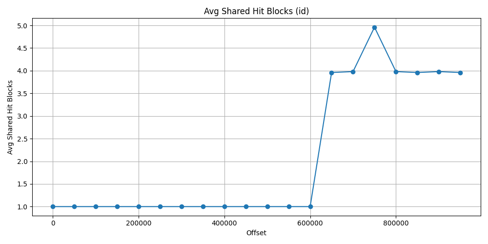
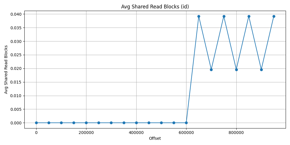
Block approach
First let’s see the id approach data. As it could be expected, due to index search first, it does not use almost any shared read block and really just a few shared hit block after 600_000 offset. The ratio is at 100% and drop just 99% at the worst situation.
| Offset | Avg Shared Hit Blocks | Avg Shared Read Blocks | Cache Hit Ratio |
|---|---|---|---|
| 0 | 1.0 | 0.0 | 1.0 |
| 50_000 | 1.0 | 0.0 | 1.0 |
| 100_000 | 1.0 | 0.0 | 1.0 |
| 150_000 | 1.0 | 0.0 | 1.0 |
| 200_000 | 1.0 | 0.0 | 1.0 |
| 250_000 | 1.0 | 0.0 | 1.0 |
| 300_000 | 1.0 | 0.0 | 1.0 |
| 350_000 | 1.0 | 0.0 | 1.0 |
| 400_000 | 1.0 | 0.0 | 1.0 |
| 450_000 | 1.0 | 0.0 | 1.0 |
| 500_000 | 1.0 | 0.0 | 1.0 |
| 550_000 | 1.0 | 0.0 | 1.0 |
| 600_000 | 1.0 | 0.0 | 1.0 |
| 650_000 | 3.960 | 0.039 | 0.990 |
| 700_000 | 3.980 | 0.019 | 0.995 |
| 750_000 | 4.960 | 0.039 | 0.992 |
| 800_000 | 3.980 | 0.019 | 0.995 |
| 850_000 | 3.960 | 0.039 | 0.990 |
| 900_000 | 3.980 | 0.019 | 0.995 |
| 950_000 | 3.960 | 0.039 | 0.990 |
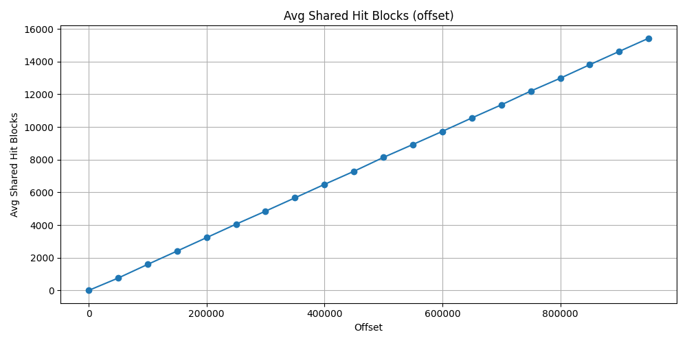
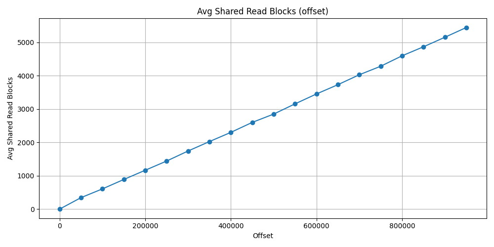
Offset approach
Shades the result, that I did not restart PostgreSQL server after each test, so the offset test has previously loaded some block to memory that has been used later test. This is why this increment can be seen in form of a linear line. Thus the cache ratio also does not goes under ~73%.
At the latest average calculation result, the shared hit block count was
15_425 and the shared read block count was 5_442.
The shared hit block size would not have been such high if the server would have
been restarted after each test. But the total block count 20867.
Which is approximately 20867*8=166936 KB => ~163MB.
This is the size of the buffers that has been used after 950_000 offset using
offset.
Meanwhile the id approach used 4 shared hit block and 0 shared read block with
same offset number. That is just 4*8=32 KB buffer usage.
| Offset | Avg Shared Hit Blocks | Avg Shared Read Blocks | Cache Hit Ratio |
|---|---|---|---|
| 0 | 1.0 | 0.0 | 1.0 |
| 50_000 | 755.745 | 343.666 | 0.687 |
| 100_000 | 1590.843 | 606.098 | 0.724 |
| 150_000 | 2407.411 | 888.333 | 0.730 |
| 200_000 | 3228.588 | 1164.686 | 0.734 |
| 250_000 | 4051.235 | 1440.647 | 0.737 |
| 300_000 | 4848.568 | 1740.980 | 0.735 |
| 350_000 | 5664.254 | 2024.078 | 0.736 |
| 400_000 | 6486.313 | 2299.568 | 0.738 |
| 450_000 | 7285.941 | 2598.666 | 0.737 |
| 500_000 | 8135.549 | 2847.705 | 0.740 |
| 550_000 | 8926.647 | 3154.196 | 0.738 |
| 600_000 | 9727.941 | 3450.490 | 0.738 |
| 650_000 | 10548.784 | 3728.313 | 0.738 |
| 700_000 | 11350.215 | 4025.705 | 0.738 |
| 750_000 | 12192.235 | 4281.254 | 0.740 |
| 800_000 | 12978.039 | 4594.058 | 0.738 |
| 850_000 | 13805.313 | 4864.333 | 0.739 |
| 900_000 | 14618.647 | 5149.921 | 0.739 |
| 950_000 | 15425.039 | 5442.137 | 0.739 |
Final words
What about UUID index or other column types?
Sometimes we use UUID as primary key. We can use UUID which is based on time
like version 7.
This gives some randomness meanwhile it depends from the actual time so it can
be in order, and can also be used with the > comparison operator on similar
way like an integer index.
In case of datetime column, if indexed, it also can be used for fast pagination.
There is no free cookie
Of course it cannot be applied for every kind of query problem. In this case I just tested it for a simple table without any join or heavier input. I just wanted to represent myself some numbers behind it, so I can see and feel the importance of indexes.
👍 My thumbs up rule that I have already learnt: always make some test query and analysis with some test data and optimize for those actions that will be rather more typically executed. For example, with more complex tables and additional indexes maybe read still fine, but every index has an amount of penalty for writing. There is always a path where we can improve ourselves and our programs.